Co-locating Prefill and Decode on One GPU: Green Contexts for Higher Throughput

CUDA Green Contexts documentation: docs.nvidia.com/cuda/cuda-programming-guide/04-special-topics/green-contexts.html

Green Contexts were released in CUDA 12.4. Their role is to split GPU resources, while the application layer still works through streams and kernels. The difference is that the submitted stream is created by a Green Context, at this time through the CUDA Driver API. In CUDA 13.1, it was exposed in the Runtime API. You can understand this as Green Contexts gradually becoming stable and starting to provide easier interfaces. In CUDA 13.3, cuBLAS started to adapt to Green Contexts and will consider the limits after Green Contexts split SMs.

It can split two kinds of GPU resources: SMs and WQs. The former can be simply understood as GPU cores. It limits how many cores a workload can use, leaving room for other workloads and avoiding the situation where a large task fills the GPU and small tasks cannot run.

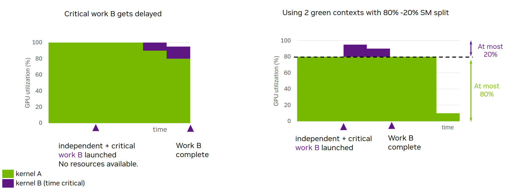
NVIDIA’s figure is very intuitive. Because there is a natural physical limit, when task B arrives, it has resources to run and can finish faster.

At this point, readers may wonder: Green Context looks like it is used to isolate fairness between multiple workloads. In inference, maybe it can isolate decode and prefill and make decode stable. But from the figure above, this causes SMs to be idle, and total performance will regress. So how did we use Green Context to improve throughput, and where did that throughput improvement come from?

Green Contexts: Very Easy to Use

The API complexity of Green Context is mainly in creation. The creation flow is roughly: configure the SM split, for example one group can use 16 SMs and another group can only use 8; allocate; create the GreenCtx; and finally create streams based on the GreenCtx. For example, if two groups are created, we get two CUDA streams: one stream can only use 16 SMs, and the other can only use 8 SMs. Apart from that, these streams are no different from normal streams. You can submit kernels normally and capture CUDA Graphs, so the application layer does not need other extra adaptation. The only thing to adapt is the creation and allocation flow, which is about seven or eight lines of code.

There are still a few adaptation points. The first one in the documentation is Thread Block Clusters. This feature was introduced from the Hopper architecture. It adds a cluster level: several blocks in the same cluster are guaranteed to be scheduled at the same time and physically placed on adjacent SMs, so DSMEM can be used. On Blackwell, TMEM and tcgen05.mma were introduced. One cluster generally equals 2, meaning two blocks. Of course, some kernels may open a very large cluster, while Green Context may be split from leftover resources. This can create a corner case, so you need to double check with cudaOccupancyMaxPotentialClusterSize.

One program can own multiple Green Contexts at the same time.

At the end, NVIDIA gives an example where Green Context improves performance. The baseline is two streams: first launch a long-running compute kernel, kernel1, on stream1; then launch a short but latency-sensitive kernel, kernel2, on stream2. Then compare that with two streams after a Green Context split, where 16 SMs are given to stream2 and 112 SMs are given to stream1, under the same pressure test.

With normal two streams, kernel1 runs for 10 ms, and kernel2 waits 1 ms before running. Its own execution time only needs 50 us.

After Green Context splitting, kernel1 needs 12 ms because it has fewer SMs, but kernel2 finishes end-to-end in only 95 us.

Inference Perspective: Prefill vs Decode

Interference, interference, and still interference. The starting point of P/D disaggregation is to keep Prefill from interrupting Decode, so that we can get stable TPOT. User output should not briefly stall because another person’s long request enters the system.

Isn’t this exactly the scenario Green Context emphasizes? Like NVIDIA’s experiment, I can give most SMs to prefill and leave some for decode. Then TPOT can be stable, although TTFT may become worse. But P/D disaggregation also makes TTFT worse because it needs transfer and rescheduling, so P/D disaggregation also has non-trivial TTFT overhead.

The question is whether this will cause idle SMs and lower total throughput, just like the previous figure.

We start with an experiment. Like NVIDIA’s experiment, we create two streams: one for a compute-intensive prefill-like workload and another for a memory-intensive decode-like workload. Then we submit 100 kernels to each stream. We compare normal two streams, Green Context two streams, and a single stream that alternates the two kernels.

We tested on both a 5070 Ti and an H200. The kernel workloads need slight adjustment between the two.

First, performance on my consumer 5070 Ti:

1. Single stream alternating two kernels: 1860 ms.
2. Naive two streams: 1812 ms, 3% faster.
3. Green Context two streams: 1173 ms, almost 60% faster than single stream.

Performance on H200:

1. Single stream: 4717 ms.
2. Naive two streams: 4446 ms, 6% faster.
3. Green Context: 3522 ms, 34% faster.

Under naive two streams, if high-priority scheduling is enabled for the stream of the memory-bound kernel and the workload construction is tuned, it can become a few percent faster, but it still cannot reach Green Context.

Look at the profiles directly. Under a single stream, the two kernels alternate as expected.

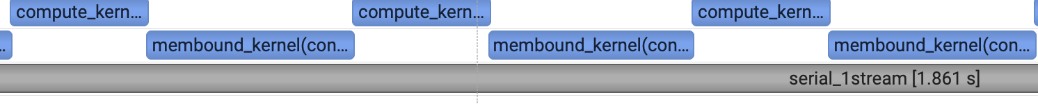
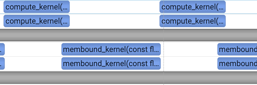
Naive two streams also alternate the two kernels.

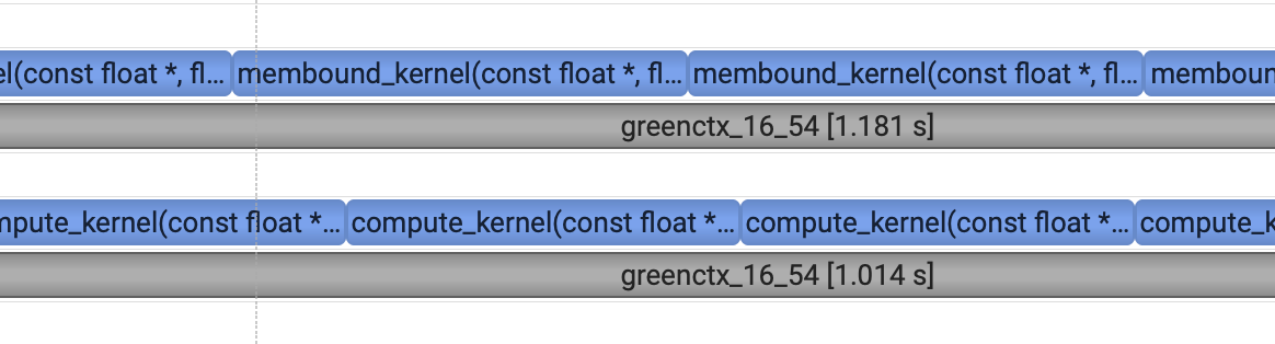
With Green Context, the two kernels become concurrent. Meanwhile, because the compute kernel is limited by fewer SMs, its time increases from 7 ms to 11 ms.

Why can two kernels running in parallel bring a performance improvement?

Why do the two-stream kernels not run in parallel? My guess is that when people normally write kernels, the grid is large by default and directly fills the GPU scheduling queue. The GPU scheduling queue is FIFO, with no preemption and no work stealing. In practice, you can also lower the SM occupancy of the kernel, which is a kind of “soft partitioning”. This makes two streams gain a bit more, but it still cannot reach Green Context.

A more aggressive way is Megakernel: launch one large kernel to schedule tasks across all SMs and implement your own scheduling logic, such as DeepSeek’s MegaMOE. In fact, people from NVIDIA in the community also gave a Green Context version of MegaMOE on Blackwell: github.com/deepseek-ai/DeepGEMM/pull/357. Its performance is not much worse than mega, and can even be faster when the data size is large.

From one angle, is Green Context another form of Megakernel?

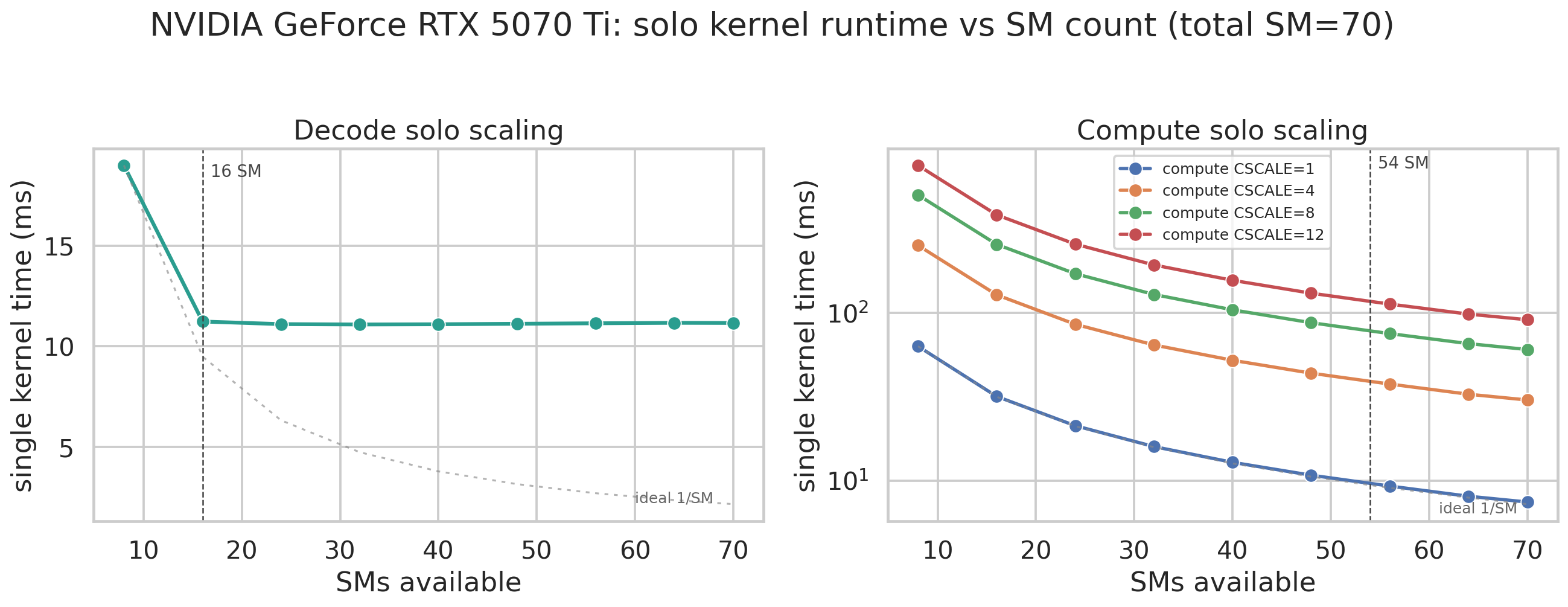
The Essence of Green Ctx Performance: SM Economics

To explain why Green Context can improve performance, we need to look separately at how decode kernels and compute kernels scale with SM count, and how their execution time changes.

On H200, it changes a bit and needs more SMs, maybe because my kernel is not written very well.

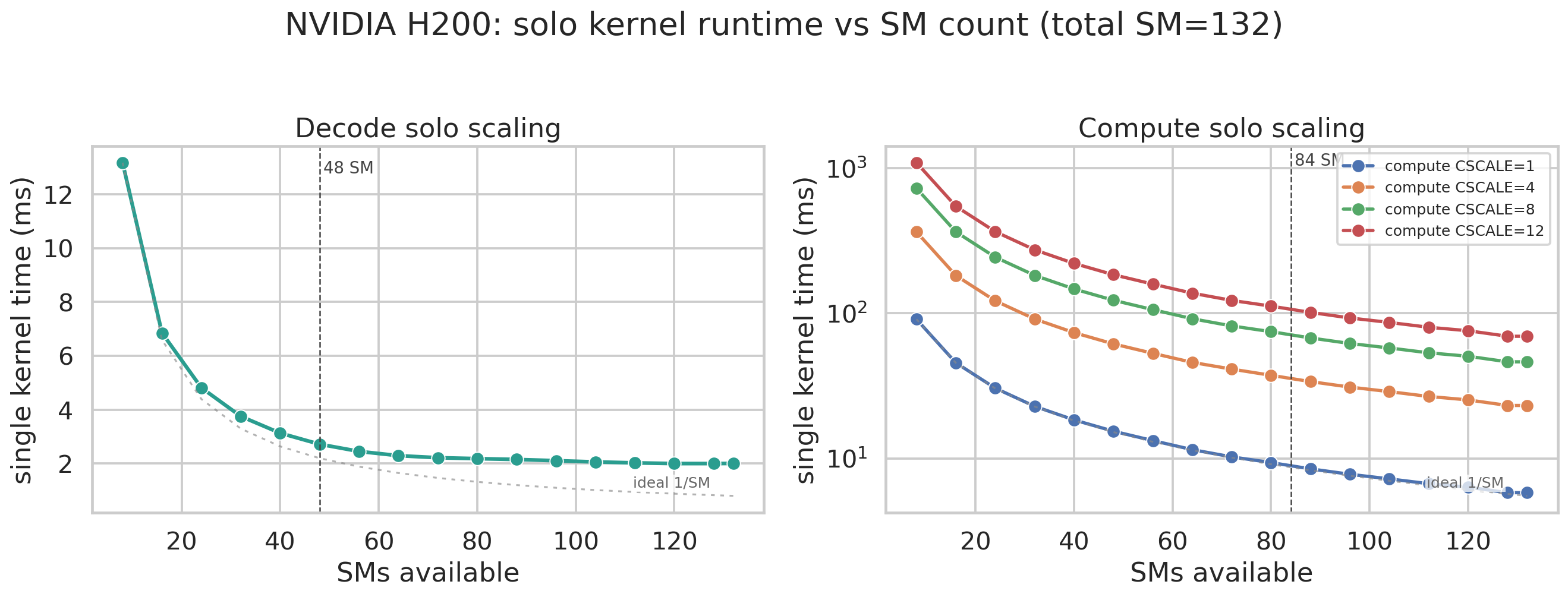
On the 5070 Ti, the memory-bound kernel no longer scales after 16 SMs. It already reaches more than 80% of theoretical bandwidth, although this case is a bit extreme. The compute kernel’s execution time almost decreases with SM growth exactly as ideally expected. H200 needs more SMs: 48 SMs are needed before it is close to a plateau, and adding more SMs afterward still gives a small improvement.

We can formalize the problem.

Input:

• The GPU has S SMs.
• There are n kinds of workloads. Each workload has prior knowledge t_i(s), the execution time of one kernel when workload i is assigned s SMs.
• Each workload has N_i kernels.

Output:

• An allocation plan {s_1, s_2, ..., s_n}, satisfying sum_i s_i <= S, and each s_i satisfies alignment or granularity constraints.
• An execution order, or concurrent orchestration, deciding which kernels run at the same time.

Objective:

• Minimize makespan C_max = max_i C_i, where C_i is the completion time of kernel i.

What kind of problem is this? We used OpenRouter’s fusion feature and let the strongest models from Opus, GPT, and Gemini discuss it together, and they reached a conclusion.

Before going through the LLM teachers’ conclusion, let’s first go through a mathematical problem called PARTITION. Suppose you and I are moving boxes. The boxes have different sizes and need different times, but one box can only be moved by one person. After all boxes are moved, both of us can leave work.

The intuition is simple: the two of us should do about the same amount of work. For example, if there are 10 identical boxes, I take 5 and you take 5. Nobody wastes time, and we leave work together. But what if there are many boxes? Another intuition is to sort the boxes by size and accumulate work until it just crosses half of the total work. But the problem is that this solution may be fine, but it is not necessarily optimal.

For example, with boxes 5 5 4 4 3 3, the total work is 24. Ideally I get 12 and you get 12, meaning each of us moves one box of size 3, 4, and 5. If sorted accumulation is used, it may allocate 3, 3, 4, 4 to me and 5, 5 to you, making it 14 and 10. That is not too bad, but it is not the optimal solution. There are also various heuristic greedy strategies, including when the number of people changes from 2 to 3. With two people it may still feel like a seesaw, but with three people it starts to become a triangle problem, and the problem becomes strongly NP-hard.

By the way, this is the mathematician’s perspective. From a programmer’s perspective, how do we treat this problem? Or rather, we actually also need to handle this kind of problem. Sometimes we do not even know the box sizes, so how do we balance it? Work stealing.

Back to our problem: “how to orchestrate SMs so all kernels finish the fastest.” The LLM teachers reached consensus that this is moldable parallel task scheduling in operations research, and a two-dimensional strip packing problem. Each kernel is a rectangle with width s_i (number of SMs) and height t_i(s_i) (time). These rectangles need to be placed without overlap inside a strip of width S, minimizing total height. It is generally NP-hard.

If it is static, it needs to be solved using ILP equivalence. This sounds high-end, but in practice it is a grouped knapsack problem.

There are n groups of items, with each kernel being one group. The backpack capacity is V = S, the total number of SMs. The s-th item in the i-th group has volume s and cost c_{i,s}. Exactly one item must be selected from each group, and the goal is to minimize total cost after putting items into the backpack.

The time complexity is the number of kernels times the square of the number of SM allocation options.

That is a bit far away, so let’s return to Green Context. Now we have found a suitable SM split ratio, or found it by brute force. The ideal time is the slowest one: ideal = max(solo_decode@memSM, solo_prefill@compSM). But what is the actual time?

When the compute kernel has high compute density, the impact is small and the time is basically the ideal value. When the compute kernel’s compute density drops, it starts to pull away from the ideal value, with at most about 10% difference. Why?

We profiled the two kernels. Metrics look like something between the two runs. For example, when the compute kernel runs alone, SM utilization is around 90%, and memory SM utilization is around 20%. When the two run concurrently, SM utilization is around 85%. DRAM and L2 hit rate also both drop, so it is hard to say which side has the larger impact.

When the compute kernel runs alone, its L2 hit rate is lower at high compute density and higher at low compute density. This means that when compute density is low, the compute kernel time may have some positive correlation with L2 hit rate.

We ran a comparison experiment. It is still a compute kernel and a memory kernel, except we shrink the working set of the memory kernel, reducing the I/O range from scanning 4 GB to scanning 4 MB.

1. Low-compute-density compute kernel: when decode scans 4 GB, it takes 16.6 ms; when decode only scans 4 MB, it takes 12.99 ms, close to the ideal value.
2. The high-compute-density compute kernel is not affected in either form.

So with this comparison experiment, we can prove one point: because decode reads a lot of data, it flushes the L2 cache, causing the low-compute-density compute kernel to slow down a lot. Maybe NVIDIA needs to add something like LRU-K or TinyLFU.

The practical problem is that we cannot reduce the decode kernel’s scan amount like this. To decode one token, the model needs to read the full weights.

On the CPU side, sometimes when we read large blocks of data, we also hope not to affect the normal CPU cache. PREFETCHNTA, Prefetch Non-Temporal Access, is designed for this: I only read this data once, so do not heavily pollute the CPU cache. It is essentially a hint. How the CPU handles it is unknown.

NVIDIA’s PTX cache operators provide several corresponding options.

Load side:

1. .ca: cache at all levels, likely to be accessed again. This is the default.
2. .cg: cache at global level, cache in L2 and below but not L1, so it does not pollute L1.
3. .cs: cache streaming, likely to be accessed once, evict first in L1 and L2.
4. .lu: last use.
5. .cv: do not cache and fetch again. It sounds like evicting L2 cache.

The store side is roughly similar, except there is no .lu.

On sm70, you can give hints to L1 cache: evict normal, evict first, evict last, evict unchanged, and no allocate, which means not using cache. They are basically normal priority, high priority, low priority, and no cache. Since they are called hints, just like on CPU, we do not know exactly what the hardware does. Support for the .level2::eviction_priority qualifier and .v8.b32 / .v4.b64 requires sm_100 or higher. Only on Blackwell can L2 evict first be used.

After enumerating decode cache policies, we can see that when running concurrently, compute starts from 24.2 ms with the default .ca; .cg worsens to 25.8 ms; .cs, L1::no_allocate / L1::evict_first, and Blackwell L2 evict first can all improve it to about 22.3 to 22.5 ms; while L2 evict last regresses to 24.7 ms. This shows that a streaming scan like decode should be marked as streaming or evict-first, avoiding one-time data staying in cache and polluting compute’s hot data.

After this optimization:

Range	Time	DRAM%	L2 hit	SM%
solo_compute	15.525 ms	23.14	20.49	83.40
concurrent_normal	16.892 ms	32.39	25.54	76.65
concurrent_cs (__ldcs / __stcs)	16.798 ms	34.57	23.32	77.08

OpenInfer Adapts Green Context

When I mention Green Context, people often ask one question: if Decode gets 20% and Prefill gets 80% of the SMs, then if the system only has Prefill or only has Decode at some moment, isn’t that wasting SMs? Even if Prefill and Decode keep arriving stably, it can only overlap one batch. Prefill may take hundreds of milliseconds, while Decode only takes tens of milliseconds. The gain may only be a few milliseconds, so it may not be necessary.

OpenInfer’s design is as follows. First, the SM split is static, for example P:D is 8:2, though different workloads and different hardware need different ratios. After the system starts, there are three streams:

1. Full-SM stream: a stream with all SMs, used for pure decode batches and prefill batches. This means that even if there is no mixed Prefill and Decode in the system, there is no performance loss.
2. Prefill-SM stream split by Green Context: used specifically to carry prefill kernels.
3. Decode-SM stream split by Green Context: used to carry decode kernels.

We capture CUDA Graphs for the full-SM stream and the decode-SM stream.

The naive scheduling algorithm is simple: if the system is pure P or pure D, tell the worker to submit to the full-SM stream. Otherwise, if it is a mixed batch, submit separately to the P stream and D stream, then wait for them to finish.

The problem is that Prefill may continue for a relatively long time, while Decode finishes quickly, causing some SMs to be idle.

The solution is also simple. The scheduler introduces two inflight batches. More simply, we make the Prefill batch asynchronous in this case. After submitting the Prefill kernel, submit a cuEvent, and then the scheduler can do a simple non-blocking query on this event. This is also one benefit Rust gives us: the worker and scheduler are in one process, so passing these things is very convenient.

When a scheduler loop observes that the event is complete, it lets the worker really trigger sync and then trigger sampling, handling the remaining work like a normal Prefill, such as committing KV blocks and submitting offloading tasks. If this request has finished Prefill, it enters the active queue, meaning the decode queue, and waits for scheduling.

The most troublesome integration problem is that GPU memory management is asynchronous. Usually, on one stream, allocation -> kernel -> release all happen on one stream, so it is safe. But now, if the kernel runs on another stream, before launching it you need to sync the stream where the first allocation happened, otherwise Xid may happen. The release timing also matters. Of course, this may be because OpenInfer has not yet given a good stream switching solution. Overall, the most troublesome point in stream switching is memory. CPU RAII and GPU RAII have a direct gap. It seems that one big pain point of io_uring is also this lifetime problem. This topic deserves another blog: how to abstract GPU resources well in Rust. There are also several experts in the Rust language community doing this kind of thing. They started companies, so maybe they are waiting for NVIDIA to acquire them.

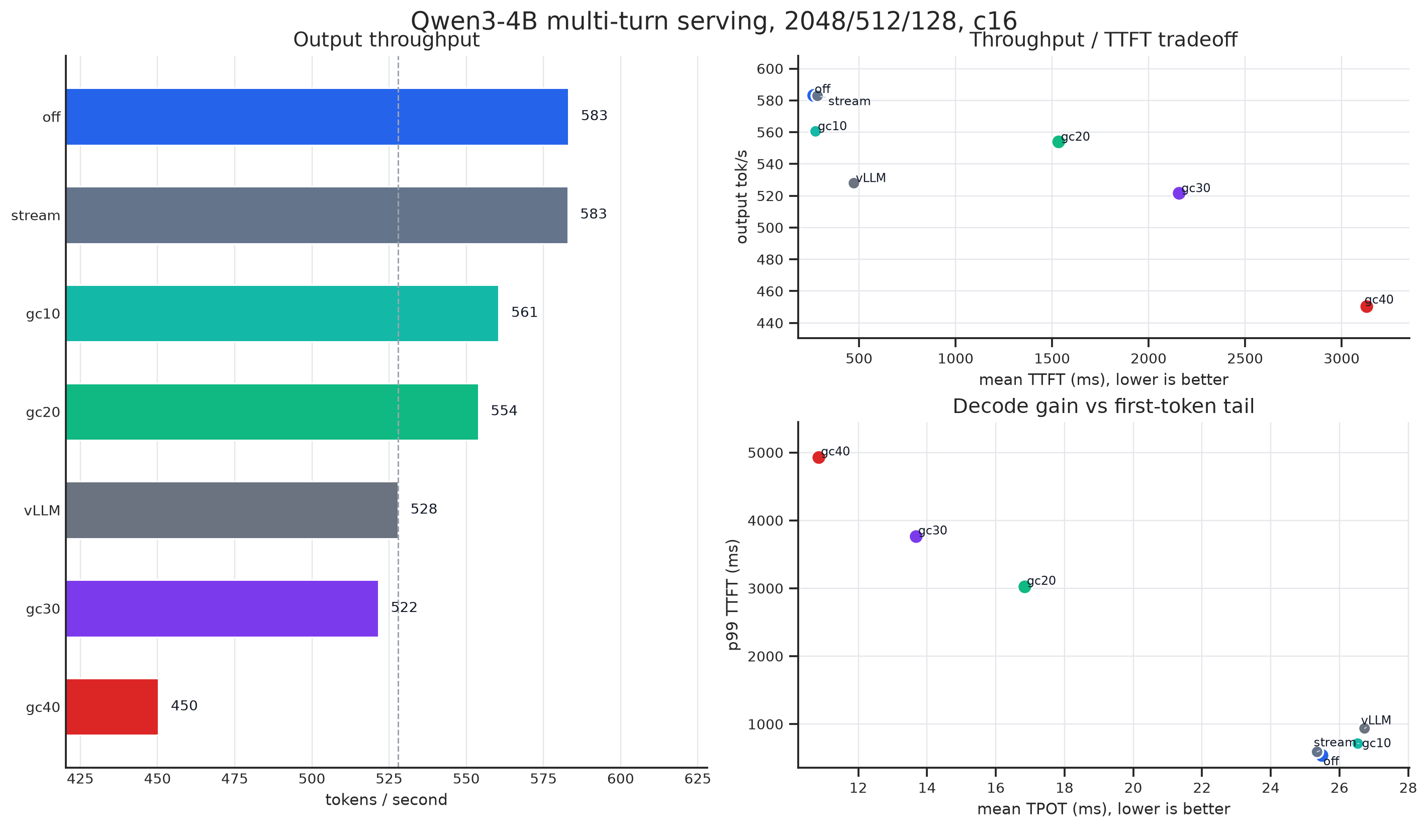
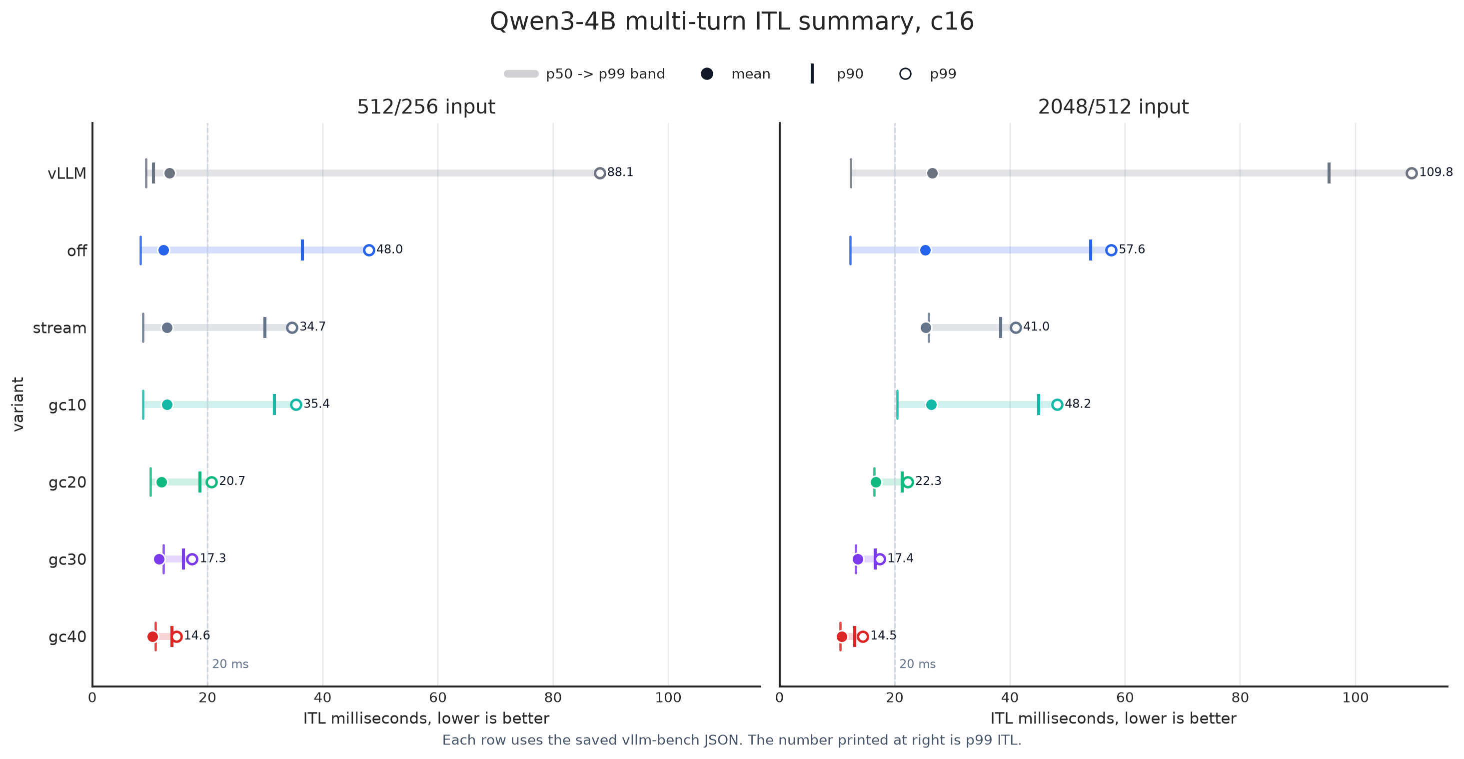
For pressure testing, we use vllm-bench, a Rust multi-turn conversation simulator that matches today’s agent workload. The pressure test is split into two groups: heavy prefill, where the first turn is 2k and later turns are 512; and light prefill, where the first turn is 512 and later turns are 256. Output is 256 tokens in both cases, with concurrency 16.

Under the heavy prefill workload, off in the figure is OpenInfer’s default stream, stream is naive two streams, and gc x% means decode uses x% of SMs.

Under the light prefill workload:

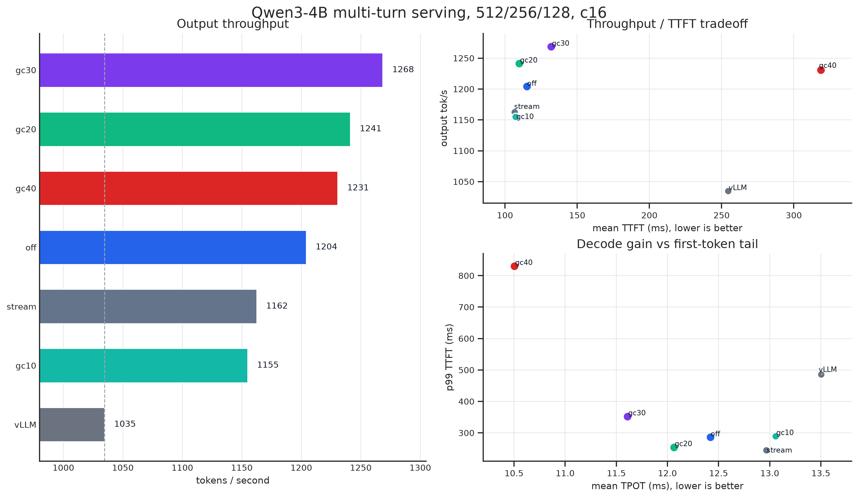
The figures already say enough. Now look at one more attractive chart: the ITL distribution. After enabling Green Context, ITL becomes extremely stable, meaning output speed is smoother.

Of course, the performance regression under the heavy prefill workload is very likely related to the L2 issue we measured earlier. Our decode kernel does not yet maintain a new set of kernels.

If heavy prefill is difficult to handle, we can still use the P/D disaggregation path, like the later Mooncake article, “Prefill As a Service.” Simply put, take long prefill out. Normal nodes only handle short prefill and decode. This is also mentioned in the Together blog, Cache-Aware Disaggregated Inference. This architecture is called CPD, an improvement over P/D. Green Context can further improve on top of CPD.

One interesting point is that after enabling Green Context, the 5090 often hits the power wall. I do not know whether commercial cards will be slightly better.

As for how to do CPD, when I was writing OpenInfer, I already had an idea: a co-design of routing, engine, and KV cache as a trinity. Now I should be fairly familiar with the second half. The engine part still has some holes to fill, including speculative decoding and then inference modeling for large MoE.

The next article will be about speculative decoding. Actually, the draft already exists: DFlash. But I will write the blog next week.