Speculative Decoding

We have already supported DFlash and DSpark speculative decoding on OpenInfer Qwen3-4B. In a ShareGPT test on a single RTX 5090, DSpark increased single-stream throughput from 170 to 381 token/s, and reduced TPOT from 5.83 ms to 2.96 ms. When concurrency is 4, throughput also increased from 576 to 1288 token/s, while keeping the output lossless.

This article will break down speculative decoding itself: how a draft model is trained, why neither draft nor verify is better when it is longer, and how the latest DSpark does dynamic verify.

Large model decode is limited by memory bandwidth: for every output token, it has to read all weights from GPU memory once. A dense model with 8GB of weights and 800GB/s bandwidth takes 10ms to read once, so the single-request limit is 100 token/s. This upper bound has nothing to do with how many requests there are, request complexity, or whether the kernel is written well. Bandwidth utilization cannot exceed the physical limit, and one forward has to read this much data. To be faster, there is only one way: make one decode forward produce more than one token.

Why can an LLM decode forward only produce one token? Mainstream LLMs are decoder-only Transformers. Attention has a causal mask, and each position can only see itself and the tokens on its left. The whole model’s training objective is “given text, predict the next token.” So in one forward, the only position that really produces something new is the last position of the sequence. It gives the distribution of the next token. The sampled token is appended back to the end of the sequence, and only then can the next forward start. The output depends on the previous step’s output, so it is naturally serial.

One intuition is: the “effort” for the model to output each token is not the same. For example, when it is writing Rust, after a newline the first token is “l” (of course the tokenizer may not split this finely), and the next tokens are very likely “e”, “t”, and then a space:

let a = 1;
let b = 2;

Is there a way to identify some pattern and guess in advance what the model may output later? The premise is that accuracy does not change: after the model gets these hints, the final output still has to be the same as the original model.

A simple idea is: before some decode step, first use some mechanism to generate several following tokens, then give them to the model for verification. If the model accepts 3 tokens, it is equivalent to one decode forward generating 3 tokens. If we temporarily ignore the extra overhead of the draft stage and the verify stage, then it is equivalent to 10ms generating 3 tokens, which means close to 3x throughput, and single-request tps changes from 100 token/s to 300 token/s.

How do we approximately measure how easy or difficult a token is to output? The model essentially outputs logits, not tokens directly. After logits are normalized, they can be understood as the model’s probability of choosing a word. For example, {"a": 0.99, "b": 0.01} means the model has a very strong tendency to choose token “a” (although this cannot be directly equivalent to difficulty). If “a” and “b” are both 0.5, it means the model also does not know what to output and has some hesitation.

We calculate entropy for the logits at every output position of the model, $H = -\sum_i p_i \log p_i$. This metric roughly represents “average uncertainty”; smaller may mean more certain.

Using Qwen3 4B as an example, we collect logits during model generation under some prompts, and observe how entropy changes when each token is output.

To clarify again, I do not think the “entropy” here can be equivalent to the difficulty the model thinks it has when outputting this token, but there should be some relationship between the two.

We look at four typical workloads.

coding comes from HumanEval. Prompt examples are:

Complete the body of this Python function. Output only the function. def has_close_elements(numbers: List[float], threshold: float) -> bool: … (with docstring + doctest, the standard OpenAI code completion style)

Write a Python function is_prime(n) that returns True if n is a prime number and False otherwise.

math comes from GSM8K.

Natalia sold clips to 48 of her friends in April, and then she sold half as many clips in May. How many clips did Natalia sell altogether in April and May?

prose source: r/WritingPrompts. We deliberately avoid famous books and let the model create freely.

Write a short story based on this writing prompt: You are the last human alive on Earth. Suddenly, you hear a knock on the door.

chat source: MT-Bench Q81 + the first Alpaca instruction.

Compose an engaging travel blog post about a recent trip to Hawaii, highlighting cultural experiences and must-see attractions.

Then we let Qwen3 4B generate greedily. For every generated token, we record logits over the whole vocabulary and calculate entropy.

Before showing the complete analysis, we first look at a concrete example from the math domain. The question is:

Natalia sold clips to 48 of her friends in April, and then she sold half as many clips in May. How many clips did Natalia sell altogether in April and May?

The model’s reply is:

Natalia sold clips to **48 friends** in **April**.

In **May**, she sold **half as many** clips as in April:

$$
\frac{48}{2} = 24
$$

So, in **May**, she sold **24 clips**.

Now, add the number of clips sold in both months:

$$
48 + 24 = 72
$$

**Answer:** Natalia sold **72 clips** altogether in April and May.

We take out the first sentence, “Natalia sold clips to 48 friends in April.”, and look at the entropy of each token in generation order (H is larger when the model hesitates more, and p1 is top-1 probability):

'N'        H=0.244 p1=0.946   # whether to restate the question first
'atal'     H=0.000 p1=1.000   # after it starts restating, entropy is very low
'ia'       H=0.000 p1=1.000
' sold'    H=0.000 p1=1.000
' clips'   H=0.050 p1=0.991
' to'      H=0.000 p1=1.000
' **'      H=0.315 p1=0.905   # whether to bold the number
'4'        H=0.000 p1=1.000   # output the number
'8'        H=0.000 p1=1.000
' friends' H=0.040 p1=0.993
'**'       H=0.074 p1=0.986
' in'      H=0.000 p1=1.000
' **'      H=0.269 p1=0.924   # still needs bold
'April'    H=0.000 p1=1.000   # repeat the question
'**'       H=0.002 p1=1.000
'.\n\n'    H=0.040 p1=0.993

For most structural outputs, such as simply restating the question or repeating numbers, once the model decides the restatement and formatting, the later output is very certain and has very low entropy. This means we most likely can use a small model to keep a high accuracy at these low-entropy positions, guess several tokens at once, and let the main model output multiple tokens in one forward.

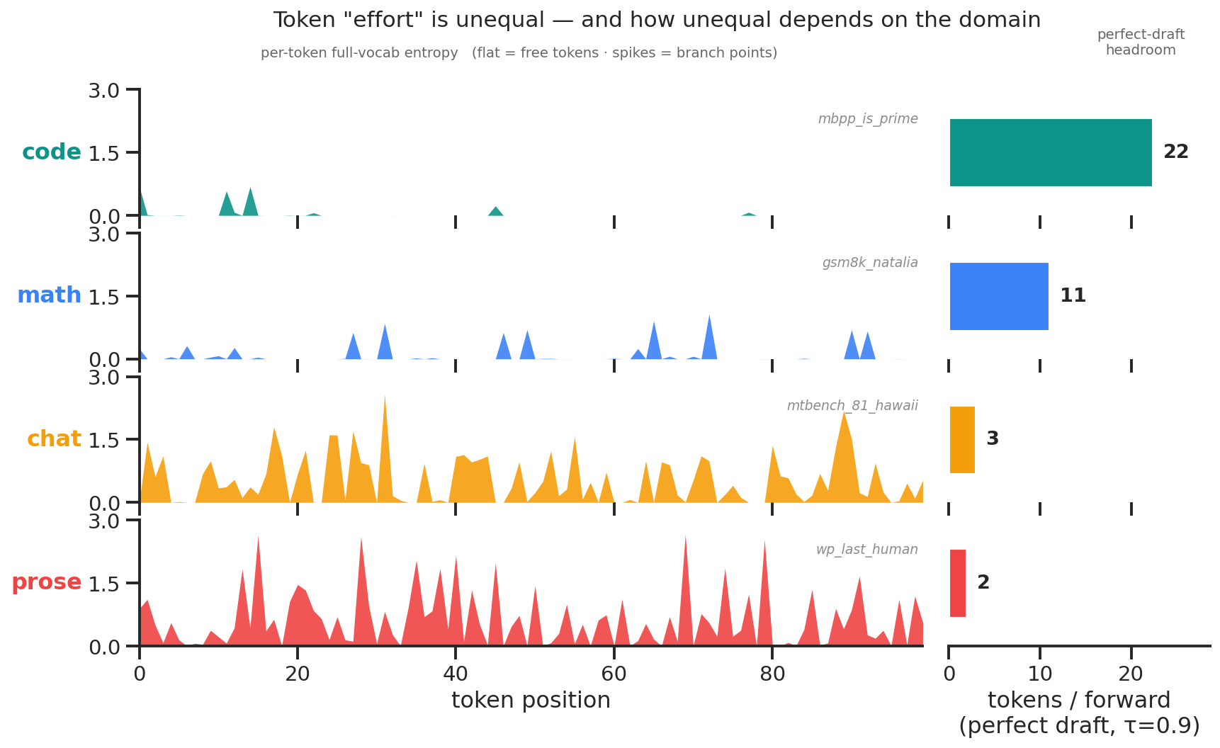
The top-left figure shows the entropy change when the model generates replies under four workloads. Code and math have lower entropy and more certain output. Chat and prose are more divergent. This shows that we may get fairly good benefits in code and math scenarios.

The top-right figure is the ideal acceleration. We mark output with top1_prob > 0.9 as positions where the model is very certain, and find such consecutive segments. For example, token 48 -> 72 is 24 consecutive tokens where the model is certain, meaning we can draft 24 tokens and send them to the model for verification. In coding and math scenarios, this number is large. In chat and prose it is only 3 and 2, but this is only a relative value.

The experiment above verifies one thing: in code and math scenarios, there are indeed many outputs with relatively low difficulty, and we can use a small model to guess them correctly.

But guessing is guessing. How exactly do we guarantee accuracy? How do we guarantee losslessness?

We start from greedy decoding, which means sampling always chooses the token with the highest probability.

Greedy verification is simple and deterministic: the target model $M$ always takes argmax, so there is a unique deterministic “standard answer” sequence: the token sequence that $M$ greedily outputs step by step. The “lossless” property of spec decode under greedy means the output is exactly the same as this standard sequence token by token, except the number of forwards of $M$ is reduced.

Starting from a real example, suppose the current context is $x_{1:t}$. In the draft stage, we use a small model $q$ to autoregressively output $\gamma$ candidate tokens $d_1,\dots,d_\gamma$. This is $\gamma$ small-model forwards and the cost is small. In the verify stage, we feed the whole sequence $[x_{1:t}, d_1, \dots, d_\gamma]$ into $M$ and run only one forward.

Why can one forward get verification for multiple positions? We use the causal mask mechanism. The causal mask says position $i$ can only see $1..i$ and cannot see the future. Technically, it presses the attention weights pointing to the future in the attention matrix to $-\infty$ (0 after softmax).

So we can put multiple draft tokens in together. The output of each position only depends on itself and the tokens to its left. With the mask, each token’s computation is no different from normal decode. For example, if 4 tokens are drafted, this forward is like processing 5 decode positions in parallel along the sequence dimension. In other words, this forward computes $\gamma+1$ distributions in parallel and isolated from each other along the sequence dimension. The hidden state at each draft token position is predicting its next token:

fed in:       x_{1:t}   d1    d2    d3    d4
                  |      |     |     |     |
predict next:    p0     p1    p2    p3    p4      <- one forward, 5 distributions

The key is that $p_i = M(\cdot \mid x_{1:t}, d_1..d_i)$ is the real conditional distribution of $M$, without any loss. The mask lets $p_i$ attend only to $x$ and $d_1..d_i$, so it equals “if $M$ were really fed this prefix, what next-token distribution would it give.” The verify step has no approximation. $M$ computes its real argmax at every position in one forward, and this is the source of losslessness.

The acceptance decision is also simple: traverse once, and compare until the first mismatch.

Using the earlier Rust example, the context stops at a newline. The greedy continuation ground truth of $M$ is let a = 1 ;, and the draft ($\gamma=4$) guessed let a = 2.

The three tokens let a = all hit. At 2, we find it is wrong, because the model chose 1 and did not choose 2. So we accept the first 3 tokens, and then take 1 as an extra reward (because it has already been forwarded and is the right choice). This round outputs let a = 1, 4 tokens / 1 forward.

So, the correctness of verification has nothing to do with how the draft came from. Whether $d_1..d_\gamma$ comes from small-model greedy, small-model sampling, n-gram copying from previous context, or random tokens, it does not affect output correctness. It only affects acceptance rate $\alpha$.

But if we add sampling, such as top-k or top-p, verification becomes a little tricky, because there is more than one legal output. Our definition of “lossless” may become: whether speculative decoding is enabled should not be perceptible at the user level; after generating many times, the two output distributions should be the same.

For example, if top_k=2 is enabled, then “a” or “b” may both be legal outputs. But if the draft only gives “b”, because it is legal, and we blindly accept it, we lose the randomness that sampling gives to the model itself. In other words, if speculative decoding and sampling are enabled at the same time, and we generate many replies for the same request, the distribution of these replies is not equivalent to the sampling result of the base model itself.

So how should we solve this problem? The first solution comes from DeepMind’s paper Accelerating Large Language Model Decoding with Speculative Sampling.

The intuition of this solution is actually not complicated. The draft keeps proposing tokens according to its own distribution $q$, while what we really want is the target distribution $p$. For each concrete token, we look at two things: how often the main model wants it, $p$, and how often the draft proposes it, $q$.

If the draft proposes it less often than the main model wants ($q < p$): this is simple. Every time it proposes, we accept it, and the remaining gap $(p-q)$ will be filled by ourselves.

Conversely, if the draft proposes it more often than we want ($q > p$): accepting all of this token must be “lossy.” So every time it proposes, we keep it only with probability $p/q$, exactly making up $p$.

In mathematical words, it is:

For one kind of good $x$, there are only two proportions:

• $p$ = the standard amount, the proportion we want.
• $q$ = the machine amount, the proportion the automatic restocking machine tends to pile up.

The key identity, one line:

$$\underbrace{\min(p,q)}_{\text{overlap}} + \underbrace{(p-q)_+}_{\text{gap}} = p$$

• Overlap $\min(p, q)$: take the smaller of the two, which is the part that the machine can supply and I also happen to want.
• Gap $(p - q)_+$: the subscript + means negative numbers become zero, which is the part I still want but the machine did not pile up enough.

Why must it hold?

• The machine piles too little ($p > q$): I accept everything the machine piles (overlap $= q$), and I fill the remaining difference myself (gap $= p - q$). Together they are exactly $p$.
• The machine piles too much ($p < q$): I have enough, and I only use as much as I need (overlap $= p$). There is no gap, so gap $= 0$. Together they are still $p$. The extra part the machine piles is not in this identity. It is the part that needs to be returned with probability during receiving, and it does not enter the shelf.

Another more engineering-oriented way, and also the current OpenInfer way: first let the main model sample one token according to its own sampling, then compare it with the token given by draft. If they are the same, accept it; if they are different, discard it. This slightly affects acceptance rate, but the measured impact is small. Unless the sampling parameters are very “open,” most of the time the model output is concentrated on a few tokens, close to greedy.

But this depends on the real workload and the real MTP, including sampling parameters received during real serving.

How to Train a Draft Model: EAGLE as an Example

The traditional or relatively naive approach is token-based, similar to a pure function: given a token list, output a token list, and predict at the token level. This approach is intuitive, but the acceptance rate is not very high.

EAGLE originally used the hidden state before logits, plus the token embedding shifted forward by one time step (that is, the token actually sampled in the previous step), as the input of the draft model. The body is a single-layer autoregressive Transformer. It directly predicts hidden states, and then still uses the main model’s lm_head to finish the hidden -> logits -> token conversion.

In this way, training is also simple: run the target LLM on training text, collect hidden states, and construct training samples. Here you can choose to let the target LLM run prefill on a real text dataset to get hidden states, or choose to let it generate answers and get hidden states from the decode stage as training data. According to the EAGLE paper, using a fixed dataset first (the answers are also from the dataset) can achieve 2.78x acceleration. If the answers are replaced by ones generated by the target itself, it can achieve 2.88x. Although there is an increase, it is not large.

The loss function is defined like this:

L = L_reg + 0.1 * L_cls

L_reg = SmoothL1(f, f_hat)

L_cls = CE(p, p_hat) = - sum_k p[k] * log(p_hat[k])

The former guarantees the accuracy of hidden state prediction, and the latter guarantees that the token distribution of the draft model is close to that of the target model. Both are for the same purpose: increasing acceptance rate. I feel this loss is not defined from first principles, which is also one motivation for later EAGLE-3.

There is another problem here: draft generation is a chain, token 1, 2, 3, 4. If token 1 is rejected, 2, 3, and 4 are all wasted. We can guess multiple tokens at one position and generate a tree, that is, multiple chains, to increase the possibility of being accepted. See this explanation.

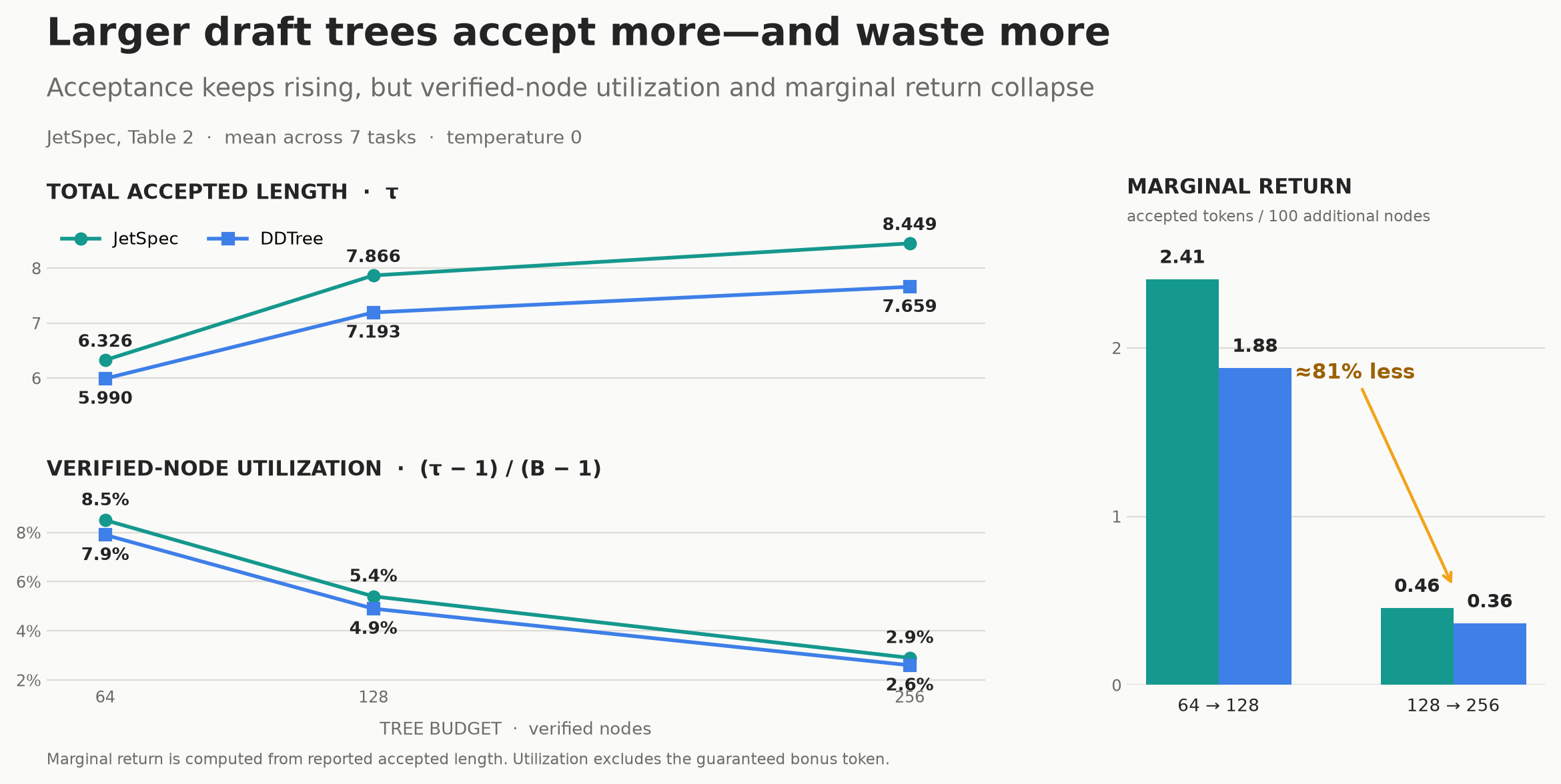
Although a tree can pull the accepted length very high and can greatly improve throughput under small batch size, a larger tree is not always better. JetSpec found that when the budget is increased from 128 to 256, the accepted tokens gained per 100 extra verification nodes are about $81\%$ less than the previous level.

EAGLE-3 takes hidden states from three layers at the same time: $l,m,h$, and then uses a fully connected layer to reduce them to “one layer,” so it obtains a feature that integrates information from different levels. At the same time, EAGLE-3’s training objective only looks at the token distribution, which makes EAGLE-3 easier to scale.

This draft can also be replaced with a diffusion model, generating multiple tokens at once, such as DFlash, which is also the DFlash that OpenInfer integrated.

DSpark’s loss also has two parts: on one hand it needs to guess accurately, and on the other hand the distribution needs to be close.

Speculative Decoding Benefit Calculation

Suppose draft generates $\gamma$ tokens at a time, and the probability that each position is accepted is $\alpha$. The first token can bring $\alpha$ expected output. The second is useful only when the first two are both accepted, so its contribution is $\alpha^2$. The contribution of the $i$-th token is $\alpha^i$. In addition, no matter where the draft fails, the target will give one correction token. Therefore the expected output of one verify round is:

$$\mathbb{E}(n) =1+\alpha+\alpha^2+\cdots+\alpha^\gamma =\frac{1-\alpha^{\gamma+1}}{1-\alpha}.$$

Simply put: the longer the draft, the harder it is for later tokens to be accepted. Every additional draft token only gives $\alpha^\gamma$ extra expected output. When $\gamma\to\infty$, total output only approaches $1/(1-\alpha)$. For example, when $\alpha=0.5$, no matter how long the draft is, one round will not exceed 2 tokens on average. When $\alpha=0.9$, the upper bound only increases to 10 tokens.

How many tokens one round can output cannot be directly equated with speedup, because generating draft and verifying both take time. Taking the time for normal decode to generate one token as 1, suppose the relative cost for the draft model to generate one token is $c$, and the relative cost for verifying $\gamma+1$ positions once is $v_\gamma$. Then one speculative decoding round costs $\gamma c+v_\gamma$ units of time. In the same time, normal decode can generate $\gamma c+v_\gamma$ tokens, while speculative decoding generates $\mathbb{E}(n)$ tokens on average. Therefore the approximate speedup is:

$$S(\gamma) \approx \frac{\mathbb{E}(n)}{\gamma c+v_\gamma} = \frac{1+\alpha+\cdots+\alpha^\gamma}{\gamma c+v_\gamma}.$$

The denominator means: every additional draft token requires paying an approximately fixed cost, and the cost may become larger as decode becomes more compute-bound (the slope increases). But the expected benefit brought by the $i$-th draft token is only $\alpha^i$. Benefits become smaller and smaller, while the cost does not disappear. When the marginal benefit of the next token cannot cover the extra draft and verify overhead it adds, continuing to lengthen draft will reduce the speedup. Therefore increasing $\gamma$ is not necessarily better, and there is usually an optimal value.

At low batch, the system is usually limited by memory bandwidth. Verify processing $\gamma+1$ positions at once takes a similar time as normal decode processing one position, namely $v_\gamma\approx1$. At this time:

$$S(\gamma)\approx\frac{1+\alpha+\cdots+\alpha^\gamma}{1+\gamma c}.$$

As long as the benefit from the first several $\alpha^i$ is greater than the extra draft cost, acceleration can be obtained. Taking $\alpha=0.9,\gamma=4,c=0.15$ as an example, the speedup is about $4.1/1.6\approx2.6$.

At high batch, the system gradually turns compute-bound, and the cost of verify increases with the number of positions, $v_\gamma\approx\gamma+1$. At this time the denominator grows approximately linearly, while the numerator gradually converges. Rejected draft tokens all become useless computation, and the speedup quickly falls below 1.

Dynamic Verify Length

After using a DFlash-style draft model, draft may no longer be the main cost. The truly expensive part is target model verify.

In a set of vLLM measurements, dynamically shortening verify length reduced acceptance length by $4.5\%$, increased throughput by $59.8\%$, and reduced TPOT by $41.2\%$.

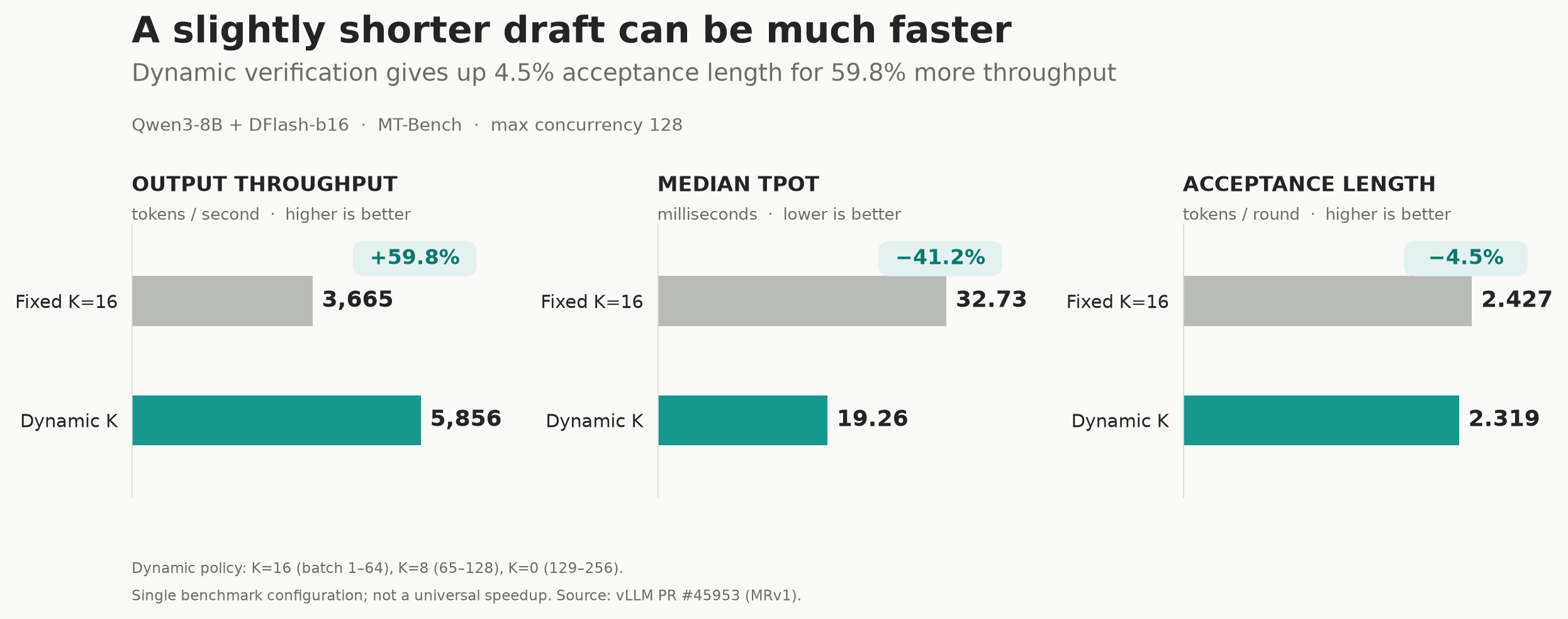
One practical solution is DSpark dynamic verify. Earlier, for convenient modeling, we assumed the acceptance probability of every position is the same $\alpha$. DSpark instead predicts acceptance probability separately for every request and every position, then dynamically decides how many of them are worth sending to the target model for verification.

Specifically, DSpark adds a confidence head on the draft model. It inputs the hidden state $h_{r,j}$ at the current position and the embedding of the previous draft token, passes them through one linear projection and sigmoid, and predicts the conditional acceptance rate of the current position:

$$c_{r,j} =\sigma\!\left(w^\top[h_{r,j};W_1[x_{r,j-1}]]\right) \approx P(\text{the }j\text{-th token is accepted}\mid\text{all previous tokens are accepted}).$$

Its training dataset also does not need to really sample many times to estimate statistics. Instead, it directly uses the distribution difference between draft and target at this position:

$$c_{r,j}^{*}=1-\frac{1}{2}\left\|p_{r,j}^{d}-p_{r,j}^{t}\right\|_1.$$

What it predicts is: under the current context and draft distribution, on average, how likely a token sampled from this position is to pass target verification.

That is the expected acceptance rate of speculative sampling at this position. Therefore every request and every draft position has one confidence, but each position only outputs one scalar.

The confidence head may be able to judge whether a token is reliable, but it may not know exactly how reliable. It reports 0.9, while the real acceptance rate may be only 0.8.

When making later decisions, $c$ needs to be multiplied cumulatively. If it is overestimated, it will amplify verify cost. So DSpark has a post-hoc calibration step, giving each position a $T$ to reduce confidence (of course, this feels like a training problem and needs algorithm people to work on it; I personally feel this solution is not very elegant).

$c_{r,j}$ is the probability that the $j$-th token itself is accepted under the condition that “all previous tokens passed.” But for the $j$-th token to really be useful, every token from the first position must pass, so its prefix survival probability is:

$$a_{r,j}=\prod_{i=1}^{j}c_{r,i}.$$

For example, if $c_{r,1}=0.9,c_{r,2}=0.8,c_{r,3}=0.7$, then the probability that the third token can really produce benefit is:

$$a_{r,3}=0.9\times0.8\times0.7=0.504.$$

How to Choose Verify Length

Suppose there are $R$ requests in the current batch, and the scheduler chooses a verification length for each request:

$$\ell_r\in\{0,\ldots,\gamma\}.$$

When request $r$ verifies $\ell_r$ draft tokens, the target model needs to process $1+\ell_r$ positions in total. The number of positions in the whole verification batch is:

$$B=\sum_{r=1}^{R}(1+\ell_r),$$

and the expected output of one round is:

$$\tau =\sum_{r=1}^{R} \left(1+\sum_{j=1}^{\ell_r}a_{r,j}\right).$$

If we only maximize $\tau$, the answer is always to send all draft tokens to verify, because this does not consider that target forward becomes slower as $B$ grows.

So we need the cost of verify. DSpark measures how many forward steps per second the target model can run under different $B$ when the engine initializes, written as $\operatorname{SPS}(B)$. This is a lookup table profiled for the current model and hardware.

What the scheduler really optimizes is system expected throughput:

$$\Theta=\tau\cdot\operatorname{SPS}(B).$$

Verifying one more token may increase expected output $\tau$, but it will also enlarge $B$ and reduce $\operatorname{SPS}(B)$. What dynamic verify wants to find is the position where the product of the two is highest.

How to Find the Optimal Length

DSpark compares candidate positions $(r,j)$ from all requests together. The marginal benefit of each position is $a_{r,j}$, and then positions are added into the verification batch one by one in descending order of $a_{r,j}$. Every time a token is added, $B$ and $\tau$ are updated, the new $\operatorname{SPS}(B)$ is queried, and $\Theta$ is calculated again.

Because it is cumulative multiplication and confidence <= 1, within the same request:

$$a_{r,j}\leq a_{r,j-1},$$

so there will not be a case where the third token of a request is selected, but its first two tokens are not selected.

In the end, high-confidence requests get longer verify prefixes, and low-confidence requests are truncated earlier.

At low load, verifying a few more tokens hardly affects $\operatorname{SPS}(B)$, so the scheduler keeps longer prefixes. After load increases, extra tokens occupy batch capacity, and the optimal verification length automatically becomes shorter.

When adding candidate tokens one by one, if it finds:

$$\Theta\leq\Theta_{\text{best}},$$

it stops expanding the verification batch. Simply put, if continuing to add tokens cannot bring higher throughput, it stops.

But sometimes the real hardware $\operatorname{SPS}(B)$ curve is not smooth. It may suddenly cross some kernel or parallelism step, and throughput becomes better instead. If it stops at the first drop, it can easily stop at a local optimum.

Later, more profile information can be maintained. The idea is similar to a database CBO: use a cost model to avoid stopping at a local optimum.